Sensitivity and discovery potential#
This tutorial demonstrates how to estimate the sensitivity and discovery potential of a point-source analysis.
Sensitivity (90 % CL): the mean number of signal events \(n_\mathrm{s}\) such that 90 % of all signal trials produce a TS value larger than the median background TS (
h0_ts_quantile=0.5,p=0.9).5σ Discovery potential: \(n_\mathrm{s}\) such that 50 % of all signal trials exceed the critical TS corresponding to a 5σ one-sided Gaussian probability (2.87e-7).
Both quantities are then converted to a flux normalization using the ana.mu2flux method of the analysis instance.
Compute time note: estimating sensitivity requires ≥ 10 000 background trials and several hundred signal trials per μ_s iteration — expect tens of minutes on a laptop. The cells below use
eps_p=0.05and a narrowmu_rangeto keep the tutorial run-time manageable while still illustrating the full workflow. For physics analyses purposes, we recommend using the defaulteps_p=0.005precision.
[1]:
import numpy as np
from matplotlib import pyplot as plt
Setup#
For analysis setup details check the Fitting a steady point-source with the public 14-year IceCube track data tutorial.
[2]:
import skyllh
from skyllh.analyses.i3.publicdata_ps.time_integrated_ps import create_analysis
from skyllh.core.config import Config
from skyllh.core.random import RandomStateService
from skyllh.core.source_model import PointLikeSource

cfg = Config()
datasets = skyllh.create_datasets('IceTracks-DR2', cfg=cfg)

src_ra = 40.67  # degrees
src_dec = -0.01  # degrees
source = PointLikeSource(ra=np.radians(src_ra), dec=np.radians(src_dec))

ana = create_analysis(cfg=cfg, datasets=datasets, source=source)
100%|██████████| 33/33 [00:00<00:00, 502.02it/s]
100%|██████████| 33/33 [00:00<00:00, 540.45it/s]
100%|██████████| 33/33 [00:00<00:00, 523.71it/s]
100%|██████████| 33/33 [00:00<00:00, 518.01it/s]
100%|██████████| 4/4 [00:45<00:00, 11.37s/it]
100%|██████████| 136/136 [00:00<00:00, 9559.99it/s]
Background trials#
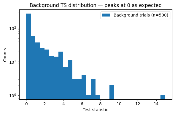
Generate background-only trials to characterise the null-hypothesis TS distribution and check that it peaks at zero (as expected for a well-behaved analysis).
The estimate_sensitivity function accepts pre-generated background trials via its h0_trials argument. If fewer trials are provided than what its internal precision criterion requires (≈ 10 000 for the default 0.5 quantile and eps_p=0.05), it will automatically extend them — so the 500 trials generated here serve as a starting point.
[4]:
rss = RandomStateService(seed=1)
bg_trials = ana.do_trials(rss=rss, n=500)

fig, ax = plt.subplots(figsize=(6, 4))
ax.hist(bg_trials['ts'], bins=30, label='Background trials (n=500)')
ax.set_xlabel('Test statistic')
ax.set_ylabel('Counts')
ax.set_yscale('log')
ax.set_title('Background TS distribution — peaks at 0 as expected')
ax.legend()
plt.tight_layout()
plt.show()
100%|██████████| 500/500 [00:37<00:00, 13.19it/s]
Sensitivity#
The estimate_sensitivity function finds the mean number of signal events μ_s such that 90 % of signal trials (injecting μ_s events on average) yield TS > TS_critical, where TS_critical is defined by the 50th percentile of the background distribution.
Key parameters:
h0_trials— pre-generated background trials (the function auto-extends if needed)h0_ts_quantile=0.5— median background TS defines the critical valuep=0.9— 90 % of signal trials must exceed the critical TSeps_p=0.05— convergence tolerance onp(default 0.005 gives tighter results but needs more trials)mu_range=(0, 15)— search range for μ_s
[5]:
from skyllh.core.utils.analysis import estimate_sensitivity

rss = RandomStateService(seed=2)
(mu_sens, mu_sens_err) = estimate_sensitivity(
    ana=ana,
    rss=rss,
    h0_trials=bg_trials,
    h0_ts_quantile=0.5,
    p=0.9,
    eps_p=0.05,
    mu_range=(0, 15),
)
flux_sens = ana.mu2flux(mu_sens)
print(f'90% CL sensitivity: mu_s = {mu_sens:.2f} signal events')
print(f'Flux sensitivity at E0=1 TeV: {flux_sens:.2e} GeV^-1 cm^-2 s^-1')
100%|██████████| 9501/9501 [11:58<00:00, 13.22it/s]
100%|██████████| 100/100 [00:09<00:00, 10.30it/s]
100%|██████████| 100/100 [00:10<00:00,  9.45it/s]
90% CL sensitivity: mu_s = 4.50 signal events
Flux sensitivity at E0=1 TeV: 1.39e-16 GeV^-1 cm^-2 s^-1
Discovery potential#
The estimate_discovery_potential function has the same interface as estimate_sensitivity but targets a different operating point: 50 % of signal trials must exceed the TS corresponding to a 5σ one-sided Gaussian probability (h0_ts_quantile=2.8665e-7, p=0.5).
Because the 5σ quantile requires very many background trials to determine directly from the tail of the TS distribution, the function automatically falls back to a truncated-gamma fit when the required trial count exceeds 500 000. This makes the background-trial requirement tractable (≈ 500 000 trials), but still makes discovery potential much slower to compute than sensitivity — expect hours of compute for a production result.
The cell below demonstrates the API; set run_discovery = True to actually execute it.
[ ]:
from skyllh.core.utils.analysis import estimate_discovery_potential

run_discovery = False  # set to True to run (takes significant compute time)

if run_discovery:
    rss = RandomStateService(seed=3)
    (mu_disc, mu_disc_err) = estimate_discovery_potential(
        ana=ana,
        rss=rss,
        h0_ts_quantile=2.8665e-7,
        p=0.5,
        eps_p=0.05,
        mu_range=(0, 50),
    )
    flux_disc = ana.mu2flux(mu_disc)
    print(f'5 sigma discovery potential: mu_s = {mu_disc:.2f} signal events')
    print(f'Discovery flux at E0=1 TeV:   {flux_disc:.2e} GeV^-1 cm^-2 s^-1')
else:
    print('Discovery potential calculation skipped (set run_discovery=True to enable).')