Fixing the Spectral Index

In this tutorial, we will show how to initialise an analysis instance with a fixed spectral index.

First, we initialize the logging, config, datasets, and source objects. Details on these can be found in the Fitting a steady point-source with the public 14-year IceCube track data and Dataset collections tutorials.

import matplotlib.pyplot as plt
import numpy as np

import skyllh
from skyllh.core.config import Config
from skyllh.core.logging import setup_logging
from skyllh.core.random import RandomStateService
from skyllh.core.source_model import PointLikeSource

cfg = Config()
logger = setup_logging(cfg=cfg, name='fixed_spectral_index')
datasets = skyllh.create_datasets('IceTracks-DR2', cfg=cfg)

# Location of NGC 1068
src_ra = 40.67  # degrees
src_dec = -0.01  # degrees

source = PointLikeSource(ra=np.radians(src_ra), dec=np.radians(src_dec))

2026-05-21 17:17:06,558 MainProcess skyllh.datasets.datasets INFO: Loaded 4 dataset(s) from sample "IceTracks-DR2": IC40, IC59, IC79, IC86_I-XI

Then we initialize the analysis object as already shown in the Fitting a steady point-source with the public 14-year IceCube track data tutorial, but we fix the seed, minimum and maximum values defining the spectral index parameter. This effectively fixes the spectral index to the desired value.

Let’s say we want to fix the spectral index to 2.0. Then we need to pass gamma_seed, gamma_min, and gamma_max equal to 2.0 to the create_analysis method.

Additionally, one would also set the refplflux_gamma parameter to the same value of 2.0, as that parameter sets the power-law spectral index that is used for generating pseudo signal events.

from skyllh.analyses.i3.publicdata_ps.time_integrated_ps import create_analysis

ana = create_analysis(
    cfg=cfg,
    datasets=datasets,
    source=source,
    refplflux_gamma=2.0,
    gamma_seed=2.0,
    gamma_min=2.0,
    gamma_max=2.0,
)

2026-05-21 17:17:07,310 MainProcess skyllh.analyses.i3.publicdata_ps.time_integrated_ps INFO: SourceHypoGroupManager
    Source Hypothesis Groups:
        0: SourceHypoGroup:
            sources (1):
                0: PointLikeSource: "4618523984": { ra=40.670 deg, dec=-0.010 deg }
            fluxmodel:
                1.000e+00 * (E / (1000 GeV))^-2 * 1 (GeV cm^2 s)^-1
            detector signal yield builders (1):
                PDSingleParamFluxPointLikeSourceI3DetSigYieldBuilder
            signal generation method:
                NoneType
2026-05-21 17:17:07,311 MainProcess skyllh.analyses.i3.publicdata_ps.time_integrated_ps INFO: ParameterModelMapper: 2 global parameters, 2 models (1 source)
    Parameters:
        ns [floating (0 <= 10 <= 1000)]
            in models:
            - IceCube: ns

        gamma [floating (2 <= 2 <= 2)]
            in models:
            - 4618523984: gamma

100%|██████████| 4/4 [00:00<00:00, 517.13it/s]
100%|██████████| 4/4 [00:00<00:00, 493.10it/s]
100%|██████████| 4/4 [00:00<00:00, 538.85it/s]
100%|██████████| 4/4 [00:00<00:00, 532.12it/s]
100%|██████████| 4/4 [00:10<00:00,  2.61s/it]
100%|██████████| 20/20 [00:00<00:00, 3740.57it/s]

As a test, we can try to fit the location of NGC 1068 with the power-law spectral index in the likelihood fixed to 2.0, which is rather far from the best-fit value we obtain when the parameter is left floating (gamma = 3.2).

The resulting TS value is much lower when the fluxmodel does not match sources spectrum (free gamma index best-fit was: TS=29.154; ns=80.09; gamma=3.21), indicating reduced statistical power.

rss = RandomStateService(seed=1)

ts, fitparam_values, status = ana.unblind(rss)

print(f'TS = {ts:.3f}')
print(f'ns = {fitparam_values["ns"]:.2f}')
print(f'gamma = {fitparam_values["gamma"]:.2f}')

TS = 2.923
ns = 9.61
gamma = 2.00

Background trials

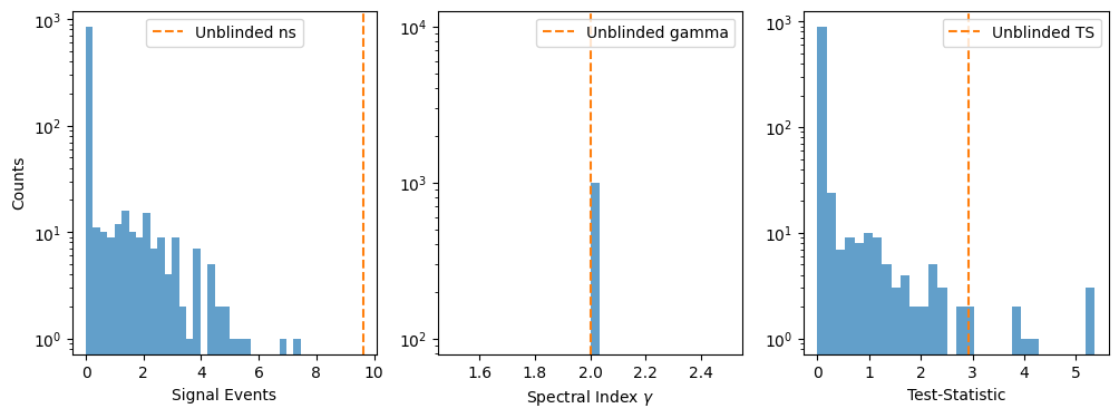
We can also check how the best fit values look of the background pseudo trials:

rss = RandomStateService(seed=1)

trials = ana.do_trials(
    rss=rss,
    n=1000,
)

100%|██████████| 1000/1000 [00:40<00:00, 24.99it/s]

fig, ax = plt.subplots(1, 3, figsize=(12, 4))

ax[0].hist(trials['ns'], bins=30, color='C0', alpha=0.7)
ax[0].axvline(fitparam_values['ns'], color='C1', linestyle='--', label='Unblinded ns')
ax[0].legend()
ax[0].set_yscale('log')
ax[0].set_ylabel(r'Counts')
ax[0].set_xlabel(r'Signal Events')

ax[1].hist(trials['gamma'], bins=30, color='C0', alpha=0.7)
ax[1].axvline(fitparam_values['gamma'], color='C1', linestyle='--', label='Unblinded gamma')
ax[1].legend()
ax[1].set_yscale('log')
ax[1].set_xlabel(r'Spectral Index $\gamma$')

ax[2].hist(trials['ts'], bins=30, color='C0', alpha=0.7)
ax[2].axvline(ts, color='C1', linestyle='--', label='Unblinded TS')
ax[2].legend()
ax[2].set_yscale('log')
ax[2].set_xlabel('Test-Statistic')
plt.show()