Time dependent analysis#
This tutorial shows how to use the public point-source data for a time dependent point-source analysis with the public IceTracks-DR2 (14-year) release, using the IC86_I-XI subset in this example. The time fit is performed by the expectation maximization (EM) algorithm.
[1]:
from matplotlib import pyplot as plt

import skyllh
from skyllh.analyses.i3.publicdata_ps.time_dependent_ps import (
    TXS_0506_PLUS056_ALERT_TIME,
    TXS_0506_PLUS056_SOURCE,
    create_analysis,
    do_trials_with_em,
    unblind_single_flare,
)
from skyllh.core.config import Config
First we need to create a local configuration for the analysis. We will create just the default configuration:
[2]:
cfg = Config()
Now we can get the dataset:
[3]:
datasets = skyllh.create_datasets('IceTracks-DR2', cfg=cfg, names=['IC86_I-XI'])
We create the Analysis instance for the TXS 0506+056 source.
The gauss argument defines the Gaussian time profile of the signal hypothesis, with which the analysis is created, i.e. its mean mu (in MJD) and its width sigma (in days). This time profile is also used when generating signal events. Here, it is centered at MJD 57000 (December 2014), close to the neutrino flare of TXS 0506+056 observed by IceCube in 2014-2015. It does not constrain the flare search below: the EM algorithm fits the time profile using the entire livetime of the data.
[4]:
ana = create_analysis(
    cfg=cfg, datasets=datasets, source=TXS_0506_PLUS056_SOURCE, refplflux_gamma=2.0, gauss={'mu': 57000, 'sigma': 65}
)
100%|██████████| 43/43 [00:00<00:00, 407.11it/s]
100%|██████████| 1/1 [01:08<00:00, 68.91s/it]
100%|██████████| 44/44 [00:00<00:00, 7913.44it/s]
[5]:
(best_ts, best_em_result, best_fitparam_values) = unblind_single_flare(ana=ana, remove_time=TXS_0506_PLUS056_ALERT_TIME)
100%|██████████| 51/51 [00:02<00:00, 17.03it/s]
[6]:
best_fitparams = ana.pmm.create_global_floating_params_dict(best_fitparam_values)

print(f'best TS = {best_ts:g}')
print(f'best em mu = {best_em_result["mu"]:g}')
print(f'best em sigma = {best_em_result["sigma"]:g}')
print(f'best ns = {best_fitparams["ns"]:g}')
print(f'best gamma = {best_fitparams["gamma"]:g}')
best TS = 15.4403
best em mu = 56966.1
best em sigma = 28.3367
best ns = 7.14054
best gamma = 2.21685
Run background trials, i.e. mean_n_sig=0
[7]:
bg_trials = do_trials_with_em(ana=ana, n=100, mean_n_sig=0, ncpu=4)
100%|██████████| 100/100 [02:00<00:00, 1.21s/it]
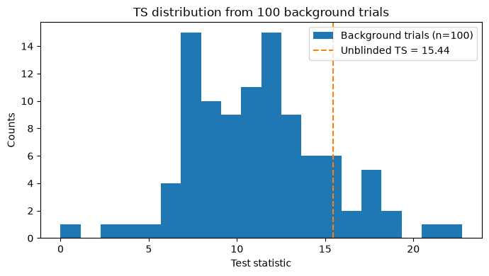
[8]:
fig, ax = plt.subplots(figsize=(7, 4))
ax.hist(bg_trials['ts'], bins=20, label='Background trials (n=100)')
ax.axvline(best_ts, color='C1', linestyle='--', label=f'Unblinded TS = {best_ts:.2f}')
ax.set_xlabel('Test statistic')
ax.set_ylabel('Counts')
ax.set_title('TS distribution from 100 background trials')
ax.legend()
plt.tight_layout()
plt.show()
Interpreting the EM parameters#
The EM algorithm fits a Gaussian time profile with two parameters:
``mu`` (MJD): the best-fit arrival time of the flare (centre of the Gaussian)
``sigma`` (days): the best-fit duration of the flare (standard deviation of the Gaussian)
Note that the IceCube alert event IceCube-170922A (MJD 58018.87, 22 September 2017), which led to the identification of TXS 0506+056, was removed from the data by the remove_time argument of unblind_single_flare. Hence, the EM algorithm finds the earlier neutrino flare of TXS 0506+056 in 2014-2015, which was found in IceCube’s archival data. Converting best_em_result["mu"] to a calendar date and comparing it with the alert time shows when this flare happened.
[9]:
from astropy.time import Time

best_mu_mjd = best_em_result['mu']
best_sigma_days = best_em_result['sigma']

best_date = Time(best_mu_mjd, format='mjd').iso
print(f'Best-fit flare time: MJD {best_mu_mjd:.1f} ({best_date})')
print(f'Best-fit flare duration (1 sigma): {best_sigma_days:.1f} days')
print(
    f'Offset from alert time (MJD {TXS_0506_PLUS056_ALERT_TIME:.2f}): '
    f'{best_mu_mjd - TXS_0506_PLUS056_ALERT_TIME:.1f} days'
)
Best-fit flare time: MJD 56966.1 (2014-11-05 01:23:36.792)
Best-fit flare duration (1 sigma): 28.3 days
Offset from alert time (MJD 58018.87): -1052.8 days
[10]:
from skyllh.core.utils.analysis import calculate_pval_from_trials

ts_vals = bg_trials['ts']
(p_val, p_val_sigma) = calculate_pval_from_trials(ts_vals, best_ts)
print(f'p-value from {len(ts_vals)} background trials: {p_val:.3f} ± {p_val_sigma:.3f}')
print()
print('Note: 100 trials is illustrative — the estimate is very noisy at this level.')
print('For a reliable p-value at TS ≈ 15, use the gamma-fit method from p_value_method_comparison.ipynb.')
p-value from 100 background trials: 0.140 ± 0.035

Note: 100 trials is illustrative — the estimate is very noisy at this level.
For a reliable p-value at TS ≈ 15, use the gamma-fit method from p_value_method_comparison.ipynb.
Applying this analysis to other sources#
To apply the time-dependent analysis to a different source:
Define a
PointLikeSourcewith the source coordinates.Call
create_analysiswith the new source and appropriate EM Gaussian priors (gauss={'mu': ..., 'sigma': ...}).Call
unblind_single_flareto find the best-fit flare parameters.Generate background trials with
do_trials_with_emand compute the p-value withcalculate_pval_from_trials.
For production-level significance estimates, generate at least a few thousand background trials.