Significance/p-value calculation#
This tutorial shows how to calculate the significance (p-value).
For this example we use the location of the blazar TXS 0506+056 as its observed TS in the time-integrated analysis is lower than the one of NGC 1068. And this makes the calculation of the corresponding p-value based on pseudo-experiment less expensive.
For analysis setup details check the Fitting a steady point-source with the public 14-year IceCube track data tutorial.
[1]:
import numpy as np
from matplotlib import pyplot as plt

import skyllh
from skyllh.analyses.i3.publicdata_ps.time_integrated_ps import create_analysis
from skyllh.core.config import Config
from skyllh.core.source_model import PointLikeSource

cfg = Config()

datasets = skyllh.create_datasets('IceTracks-DR2', cfg=cfg)

# Location of the blazar TXS 0506+056
src_ra = 77.35  # degrees
src_dec = 5.7  # degrees

source = PointLikeSource(ra=np.radians(src_ra), dec=np.radians(src_dec))

ana = create_analysis(cfg=cfg, datasets=datasets, source=source)
100%|██████████| 33/33 [00:00<00:00, 513.21it/s]
100%|██████████| 33/33 [00:00<00:00, 521.56it/s]
100%|██████████| 33/33 [00:00<00:00, 531.66it/s]
100%|██████████| 33/33 [00:00<00:00, 514.15it/s]
100%|██████████| 4/4 [00:23<00:00,  5.81s/it]
100%|██████████| 136/136 [00:00<00:00, 9478.65it/s]
Initializing the analysis instance and unblinding the data.
[2]:
from skyllh.core.random import RandomStateService

rss = RandomStateService(3090)
ts, fitparam_values, status = ana.unblind(rss)
ns_bf = fitparam_values['ns']
gamma_bf = fitparam_values['gamma']
print(f'Unblinded results: TS={ts:.2f}, ns={ns_bf:.2f}, gamma={gamma_bf:.2f}')
print(f'Minimizer status: {status}')
Unblinded results: TS=9.72, ns=8.88, gamma=1.98
Minimizer status: {'grad': array([-3.24275493e-06,  5.29904401e-05]), 'task': 'CONVERGENCE: RELATIVE REDUCTION OF F <= FACTR*EPSMCH', 'funcalls': 18, 'nit': 14, 'warnflag': 0, 'skyllh_minimizer_n_reps': 0, 'n_llhratio_func_calls': 18}
Calculating the significance (local p-value) by generating the test-statistic distribution of background-only pseudo-experiments (trials)#
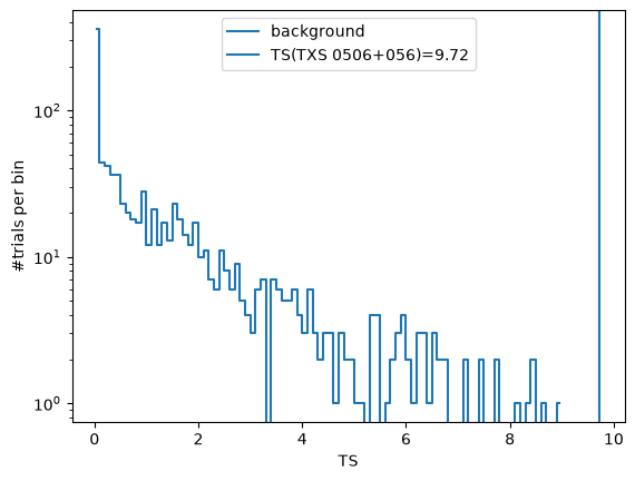
The local significance of the source, i.e. its p-value, can be calculated by generating the test-statistic distribution of background-only pseudo-experiments, i.e. for zero injected signal events. SkyLLH provides the helper function create_trial_data_file to generate these trials and store them in a numpy file for later usage.
[3]:
from skyllh.core.utils.analysis import create_trial_data_file
[4]:
help(create_trial_data_file)
Help on function create_trial_data_file in module skyllh.core.utils.analysis:

create_trial_data_file(
    ana: Analysis,
    rss: RandomStateService,
    n_trials: int,
    mean_n_sig=0,
    mean_n_sig_null=0,
    mean_n_bkg_list: list[float] | None = None,
    minimizer_rss: RandomStateService | None = None,
    bkg_kwargs: dict | None = None,
    sig_kwargs: dict | None = None,
    pathfilename: str | None = None,
    ncpu: int | None = None,
    ppbar: ProgressBar | None = None,
    tl: TimeLord | None = None
) -> tuple[int, np.ndarray, np.ndarray, np.ndarray]
    Creates and fills a trial data file with `n_trials` generated trials for
    each mean number of injected signal events specified by `mean_n_sig` for a
    given analysis.

    Parameters
    ----------
    ana
        The Analysis instance to use for the trial generation.
    rss
        The RandomStateService instance to use for generating random
        numbers.
    n_trials
        The number of trials to perform for each hypothesis test.
    mean_n_sig
        The array of mean number of injected signal events (MNOISEs) for which
        to generate trials. If this argument is not a ndarray, an array of
        MNOISEs is generated based on this argument.
        If a single float is given, only this given MNOISEs are injected.
        If a 2-element sequence of floats is given, it specifies the range of
        MNOISEs with a step size of one.
        If a 3-element sequence of floats is given, it specifies the range plus
        the step size of the MNOISEs.
    mean_n_sig_null
        The array of the fixed mean number of signal events (FMNOSEs) for the
        null-hypothesis for which to generate trials. If this argument is not a
        ndarray, an array of FMNOSEs is generated based on this argument.
        If a single float is given, only this given FMNOSEs are used.
        If a 2-element sequence of floats is given, it specifies the range of
        FMNOSEs with a step size of one.
        If a 3-element sequence of floats is given, it specifies the range plus
        the step size of the FMNOSEs.
    mean_n_bkg_list
        The mean number of background events that should be generated for
        each dataset. This parameter is passed to the ``do_trials`` method of
        the ``Analysis`` class. If set to None (the default), the background
        generation method needs to obtain this number itself.
    minimizer_rss
        The instance of RandomStateService to use for generating random
        numbers for the minimizer, e.g. new initial fit parameter values.
        If set to ``None``, a rss with the same seed as ``rss`` will be
        initialized.
    bkg_kwargs
        Additional keyword arguments for the `generate_events` method of the
        background generation method class. An usual keyword argument is
        `poisson`.
    sig_kwargs
        Additional keyword arguments for the `generate_signal_events` method
        of the `SignalGenerator` class. An usual keyword argument is
        `poisson`.
    pathfilename
        Trial data file path including the filename.
        If set to None generated trials won't be saved.
    ncpu
        The number of CPUs to use.
    ppbar
        The optional instance of the parent progress bar.
    tl
        The instance of TimeLord that should be used to measure individual
        tasks.

    Returns
    -------
    seed
        The seed used to generate the trials.
    mean_n_sig
        The array holding the mean number of signal events used to generate the
        trials.
    mean_n_sig_null
        The array holding the fixed mean number of signal events for the
        null-hypothesis used to generate the trials.
    trial_data
        The generated trial data.
[5]:
from skyllh.core.timing import TimeLord

tl = TimeLord()

# The number of CPU cores to use for generating the trials.
ncpu = 8
[6]:
rss = RandomStateService(seed=1)
(_, _, _, trials) = create_trial_data_file(
    ana=ana, rss=rss, n_trials=1000, mean_n_sig=0, pathfilename='txs_bkg_trials.npy', ncpu=ncpu, tl=tl
)
print(tl)
100%|██████████| 1001/1001 [00:17<00:00, 56.05it/s]
TimeLord: Executed tasks:
[Generating background events for dataset "IC40".     ] 6.5e-04 sec/iter (1000)
[Generating background events for dataset "IC59".     ]   0.001 sec/iter (1000)
[Generating background events for dataset "IC79".     ]   0.001 sec/iter (1000)
[Generating background events for dataset "IC86_I-XI".]   0.008 sec/iter (1000)
[Generating pseudo data.                              ]   0.010 sec/iter (1000)
[Initializing trial.                                  ]   0.018 sec/iter (1000)
[Get sig probability densities and grads.             ] 1.1e-06 sec/iter (88192)
[Get bkg probability densities and grads.             ] 7.5e-07 sec/iter (88192)
[Calculate PDF ratios.                                ] 4.5e-05 sec/iter (88192)
[Calc pdfratio value Ri                               ] 3.4e-04 sec/iter (44096)
[Calc logLambda and grads                             ] 1.1e-04 sec/iter (44096)
[Evaluate llh-ratio function.                         ]   0.002 sec/iter (11024)
[Minimize -llhratio function.                         ]   0.018 sec/iter (1000)
[Maximizing LLH ratio function.                       ]   0.018 sec/iter (1000)
[Calculating test statistic.                          ] 1.2e-05 sec/iter (1000)
After generating the background trials, we can histogram the test-statistic values and plot the TS distribution.
[7]:
fig, ax = plt.subplots()
(h, be) = np.histogram(trials['ts'], bins=np.arange(0, np.max(trials['ts']) + 0.1, 0.1))
ax.plot(0.5 * (be[:-1] + be[1:]), h, drawstyle='steps-mid', label='background')
ax.axvline(ts, label=f'TS(TXS 0506+056)={ts:.2f}')
ax.set_yscale('log')
ax.set_xlabel('TS')
ax.set_ylabel('#trials per bin')
ax.legend()
plt.show()
One can also use a helper function extend_trial_data_file to extend the trial data if the trial data generated is not enough to estimate the p-value reliably.
[8]:
from skyllh.core.utils.analysis import extend_trial_data_file
[9]:
help(extend_trial_data_file)
Help on function extend_trial_data_file in module skyllh.core.utils.analysis:

extend_trial_data_file(
    ana: Analysis,
    rss: RandomStateService,
    n_trials: int,
    trial_data: np.ndarray,
    mean_n_sig=0,
    mean_n_sig_null=0,
    mean_n_bkg_list=None,
    bkg_kwargs: dict | None = None,
    sig_kwargs: dict | None = None,
    pathfilename: str | None = None,
    **kwargs
)
    Appends to the trial data file `n_trials` generated trials for each
    mean number of injected signal events specified by `mean_n_sig` for a
    given analysis.

    Parameters
    ----------
    ana
        The Analysis instance to use for sensitivity estimation.
    rss
        The RandomStateService instance to use for generating random
        numbers.
    n_trials
        The number of trials the trial data file needs to be extended by.
    trial_data
        The structured numpy ndarray holding the trials.
    mean_n_sig
        The array of mean number of injected signal events (MNOISEs) for which
        to generate trials. If this argument is not a ndarray, an array of
        MNOISEs is generated based on this argument.
        If a single float is given, only this given MNOISEs are injected.
        If a 2-element sequence of floats is given, it specifies the range of
        MNOISEs with a step size of one.
        If a 3-element sequence of floats is given, it specifies the range plus
        the step size of the MNOISEs.
    mean_n_sig_null
        The array of the fixed mean number of signal events (FMNOSEs) for the
        null-hypothesis for which to generate trials. If this argument is not a
        ndarray, an array of FMNOSEs is generated based on this argument.
        If a single float is given, only this given FMNOSEs are used.
        If a 2-element sequence of floats is given, it specifies the range of
        FMNOSEs with a step size of one.
        If a 3-element sequence of floats is given, it specifies the range plus
        the step size of the FMNOSEs.
    bkg_kwargs
        Additional keyword arguments for the `generate_events` method of the
        background generation method class. An usual keyword argument is
        `poisson`.
    sig_kwargs
        Additional keyword arguments for the `generate_signal_events` method
        of the `SignalGenerator` class. An usual keyword argument is
        `poisson`.
    pathfilename
        Trial data file path including the filename.

    Additional keyword arguments
    ----------------------------
    Additional keyword arguments are passed-on to the ``create_trial_data_file``
    function.

    Returns
    -------
    trial_data :
        Trial data file extended by the required number of trials for each
        mean number of injected signal events..
[10]:
tl = TimeLord()
rss = RandomStateService(seed=2)
trials = extend_trial_data_file(
    ana=ana, rss=rss, n_trials=4000, trial_data=trials, pathfilename='txs_bkg_trials.npy', ncpu=ncpu, tl=tl
)
100%|██████████| 4001/4001 [01:12<00:00, 55.26it/s]
[11]:
print(tl)
TimeLord: Executed tasks:
[Generating background events for dataset "IC40".     ] 6.3e-04 sec/iter (4000)
[Generating background events for dataset "IC59".     ]   0.001 sec/iter (4000)
[Generating background events for dataset "IC79".     ]   0.001 sec/iter (4000)
[Generating background events for dataset "IC86_I-XI".]   0.008 sec/iter (4000)
[Generating pseudo data.                              ]   0.009 sec/iter (4000)
[Initializing trial.                                  ]   0.016 sec/iter (4000)
[Get sig probability densities and grads.             ] 1.1e-06 sec/iter (343864)
[Get bkg probability densities and grads.             ] 7.5e-07 sec/iter (343864)
[Calculate PDF ratios.                                ] 4.4e-05 sec/iter (343864)
[Calc pdfratio value Ri                               ] 3.1e-04 sec/iter (171932)
[Calc logLambda and grads                             ] 1.1e-04 sec/iter (171932)
[Evaluate llh-ratio function.                         ]   0.001 sec/iter (42983)
[Minimize -llhratio function.                         ]   0.016 sec/iter (4000)
[Maximizing LLH ratio function.                       ]   0.016 sec/iter (4000)
[Calculating test statistic.                          ] 1.2e-05 sec/iter (4000)
Among utility functions saved in the library skyllh.core.utils.analysis, SkyLLH offers a function calculate_pval_from_trials that allows one to calculate the p-value empirically directly from the distribution of background trials. The function takes the created background-only pseudo-experiments and the observed TS value and it returns the corresponding p-value and the related statistical uncertainty.
[12]:
from skyllh.core.utils.analysis import calculate_pval_from_trials
[13]:
help(calculate_pval_from_trials)
Help on function calculate_pval_from_trials in module skyllh.core.utils.analysis:

calculate_pval_from_trials(
    ts_vals: np.ndarray,
    ts_threshold: float,
    comp_operator: str = 'greater_equal'
) -> tuple[float, float]
    Calculates the percentage (p-value) of test-statistic trials that are
    above the given test-statistic critical value.
    In addition it calculates the standard deviation of the p-value assuming
    binomial statistics.

    Parameters
    ----------
    ts_vals
        The ndarray holding the test-statistic values of the trials.
    ts_threshold
        The critical test-statistic value.
    comp_operator
        The comparison operator for p-value calculation. It can be set to one of
        the following options: 'greater' or 'greater_equal'.

    Returns
    -------
    p, p_sigma: tuple(float, float)
[14]:
trials = np.load('txs_bkg_trials.npy')
[15]:
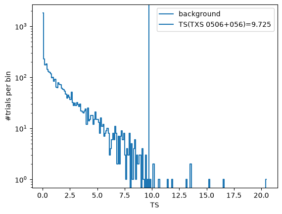
p_val_from_trials, p_val_from_trials_sigma = calculate_pval_from_trials(trials['ts'], ts)
print(f'p_value calculated from trials: {p_val_from_trials:.3e}')
p_value calculated from trials: 2.400e-03
Here below we provide a visualization of the computed background-only pseudo-experiments TS values together with the observed TS for TXS 0506+056
[16]:
fig, ax = plt.subplots()
(h, be) = np.histogram(trials['ts'], bins=np.arange(0, np.max(trials['ts']) + 0.1, 0.1))
ax.plot(0.5 * (be[:-1] + be[1:]), h, drawstyle='steps-mid', label='background')
ax.axvline(ts, label=f'TS(TXS 0506+056)={ts:.3f}')
ax.set_yscale('log')
ax.set_xlabel('TS')
ax.set_ylabel('#trials per bin')
ax.legend()
plt.show()
Calculating the significance (local p-value) by fitting a truncated gamma function#
It can happen (if you’re lucky or if you’re estimating a \(5\sigma\) discovery potential, see the Sensitivity study notebook) that the observed TS is high enough that computing background trials to calculate the corresponding p-value becomes extremely expensive.
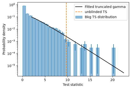
While the empirical estimation remains the most robust way to compute a significance, a faster alternative is to fit the tail of the generated distribution of background-only pseudo-experiments with a truncated gamma function and use it to extrapolate p-values at higher TS values.
Among the analysis utility functions, SkyLLH offers the fit_truncated_gamma function, which fits the truncated gamma function to the TS distribution.
Additionally, the calculate_pval_from_gammafit_to_trials function provides a wrapper method that runs the fit and returns the p-value estimated from the fit.
Note
Fitting the truncated gamma function requires the iminuit Python package, which can be installed via
pip install "skyllh[extras]".
[17]:
from scipy.stats import gamma

from skyllh.core.utils.analysis import (
    calculate_critical_ts_from_gamma,
    calculate_pval_from_gammafit_to_trials,
    fit_truncated_gamma,
)
You need to truncate the distribution at some \(\eta > 0\) because the TS distribution is the sum of a delta peak at 0 and a continuous distribution for TS > 0. Here we choose \(\eta=2.0\).
[18]:
eta = 2.0
pars, norm = fit_truncated_gamma(trials['ts'], eta=eta)

# Plot
fig, ax = plt.subplots(1, 1, figsize=(6, 4))
bins = np.linspace(0, np.max(trials['ts']) + 0.1, 30)
counts, _ = np.histogram(trials['ts'], bins=bins, density=True)
ax.bar(
    0.5 * (bins[1:] + bins[:-1]),
    height=counts,
    width=bins[1:] - bins[:-1],
    edgecolor='C0',
    color='C0',
    alpha=0.5,
    label='Bkg TS distribution',
)
ax.errorbar(
    0.5 * (bins[1:] + bins[:-1]),
    counts,
    yerr=np.sqrt(counts / len(trials['ts']) / (bins[1:] - bins[:-1])),
    fmt='',
    ls='',
    color='C0',
)
ax.set_yscale('log')

vals = np.linspace(eta, np.max(trials['ts']) + 2, 100)
ax.plot(
    vals, norm * gamma.pdf(vals, a=pars[0], scale=pars[1]), lw=1.5, color='k', zorder=5, label='Fitted truncated gamma'
)

ax.axvline(ts, color='C1', linestyle='--', label='unblinded TS')

ax.set_xlabel('Test statistic')
ax.set_ylabel('Probability density')

ax.legend()
plt.show()
calculate_critical_ts_from_gamma function calculates the TS you would need in your analysis to reach a given significance. We use the same truncation value \(\eta\) as for the fit above.
[19]:
critical_ts = calculate_critical_ts_from_gamma(
    ts=trials['ts'],
    h0_ts_quantile=1.3e-3,  # this is ~ 3 sigma
    eta=eta,
)
print(f'TS value for a 3 sigma detection: {critical_ts:.2f}')
critical_ts = calculate_critical_ts_from_gamma(
    ts=trials['ts'],
    h0_ts_quantile=2.9e-7,  # this is ~ 5 sigma
    eta=eta,
)
print(f'TS value for a 5 sigma detection: {critical_ts:.2f}')
TS value for a 3 sigma detection: 12.10
TS value for a 5 sigma detection: 27.52
And of course you can also calculate the p-value for the observed TS from the fitted function. This should result in a p-value of the same order of magnitude as the one estimated empirically from the trials.
[20]:
p_val_from_fit, _ = calculate_pval_from_gammafit_to_trials(trials['ts'], ts, eta=eta)
print(f'p_value calculated from fit: {p_val_from_fit:.3e}')
p_value calculated from fit: 4.595e-03
Practically, one might be interested in flip-flopping from one estimation method to the other depending on how high the TS value of interest is and on how many pseudo-experiments have been computed to populate the background TS distribution.
This feature exists in the calculate_pval_from_trials_mixed method, which takes a switch_at_ts additional argument to set at what TS value one should switch from the empirical estimation to the evaluation of the truncated gamma fit.
[21]:
from skyllh.core.utils.analysis import calculate_pval_from_trials_mixed

# The observed TS is above switch_at_ts, hence the p-value is taken from the truncated gamma fit.
p_val_mixed, _ = calculate_pval_from_trials_mixed(trials['ts'], ts, switch_at_ts=eta, eta=eta)
print(f'p_value calculated with the mixed method (switch_at_ts={eta}): {p_val_mixed:.3e}')

# The observed TS is below switch_at_ts, hence the p-value is calculated from the trials directly.
p_val_mixed, _ = calculate_pval_from_trials_mixed(trials['ts'], ts, switch_at_ts=20.0, eta=eta)
print(f'p_value calculated with the mixed method (switch_at_ts=20.0): {p_val_mixed:.3e}')
p_value calculated with the mixed method (switch_at_ts=2.0): 4.595e-03
p_value calculated with the mixed method (switch_at_ts=20.0): 2.400e-03