Setting a user-defined energy range for the signal injection

This tutorial shows how to set an energy range for the signal injection and how to visualize the distribution of the generated pseudo-data events.

First, we initialize the logging, config, datasets, and source objects. Details on these can be found in the Fitting a steady point-source with the public 14-year IceCube track data and Dataset collections tutorials.

import matplotlib.pyplot as plt
import numpy as np

import skyllh
from skyllh.core.config import Config
from skyllh.core.logging import setup_logging
from skyllh.core.source_model import PointLikeSource

cfg = Config()
logger = setup_logging(cfg=cfg, name='setting_an_energy_range')
datasets = skyllh.create_datasets('IceTracks-DR2', cfg=cfg)

# Location of NGC 1068
src_ra = 40.67  # degrees
src_dec = -0.01  # degrees

source = PointLikeSource(ra=np.radians(src_ra), dec=np.radians(src_dec))

2026-05-13 19:34:56,733 MainProcess skyllh.datasets.datasets INFO: Loaded 4 dataset(s) from sample "IceTracks-DR2": IC40, IC59, IC79, IC86_I-XI

The create_analysis instance can be created with the energy_range set to a specific energy range. This interanlly sets the energy range for the singal generator. Here in this example, the analysis object is created with the energy range \(10^2\, \text{GeV}\) to \(10^3\, \text{GeV}\).

from skyllh.analyses.i3.publicdata_ps.time_integrated_ps import create_analysis

ana = create_analysis(cfg=cfg, datasets=datasets, source=source, energy_range=(1e2, 1e3))

100%|██████████| 33/33 [00:17<00:00,  1.90it/s]
100%|██████████| 33/33 [00:17<00:00,  1.89it/s]
100%|██████████| 33/33 [00:05<00:00,  5.87it/s]
100%|██████████| 33/33 [00:08<00:00,  3.73it/s]
100%|██████████| 4/4 [04:04<00:00, 61.14s/it]
100%|██████████| 136/136 [00:00<00:00, 2145.34it/s]

The ana instance has a generate_signal_events method, which can be used to generate signal-like pseudo-data. The function takes the RandomStateService instance and the mean number of events to be generated as its arguments along with a few optional arguments. The actual number of generated events is drawn from a Poisson distribution with mean value mean_n_sig.

It returns:

1. The actual number of generated events;

2. The list of the number of signal events that have been generated for each data set;

3. The list of instance of DataFieldRecordArray containing the signal data events for each data set. An entry is None, if no signal events were generated for this particular data set.

Here below we generate 100 signal-like events:

help(ana.generate_signal_events)

from skyllh.core.random import RandomStateService

mean_n_sig = 100

rss = RandomStateService(seed=1)
n_sig_erange, n_events_list_erange, events_list_erange = ana.generate_signal_events(rss=rss, mean_n_sig=mean_n_sig)

It is also possible to change the energy range to generate signal events without having to reinitialise the analysis instance ana. By re-defining ana.energy_range, one can change what ana.generate_signal_events() uses as the energy range.

By setting ana.energy_range to None, we fall back to the full energy range of the analysis, which is the maximum energy range covered in the smearing matrix, that is (1e2 - 1e9) GeV.

rss = RandomStateService(seed=1)
ana.energy_range = None
n_sig, n_events_list, events_list = ana.generate_signal_events(rss=rss, mean_n_sig=mean_n_sig)

Now we can look at the true neutrino energy of the generate pseudo-data events and check that they belong to their respective energy ranges.

print(events_list[0])

log_true_energy = np.concatenate([events['log_true_energy'] for events in events_list])
injected_log_true_energy = np.concatenate([events['log_true_energy'] for events in events_list_erange])

bins = np.linspace(2, 9, 56)
plt.hist(log_true_energy, bins=bins, histtype='step', label='Signal events without any energy range cuts')
plt.hist(
    injected_log_true_energy,
    bins=bins,
    histtype='step',
    label='Signal events with (1e2, 1e3) GeV energy range cut',
)
plt.title('Generated signal events with gamma=2.0')
plt.xlabel('Log True Energy [GeV]')
plt.ylabel('Number of generated events')
plt.grid('True')
plt.legend()
plt.show()

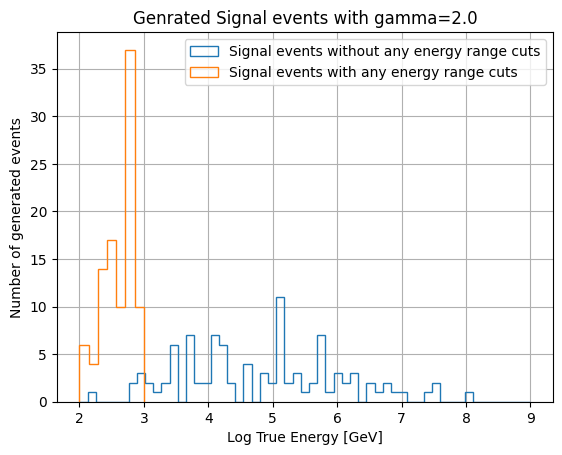
It is to be noted that the only thing that is being limited is the injected signal: We inject signals only in that energy range but the signal hypothesis in the likelihood still assumes the full energy range.