PISA stage modes

Every PISA stage of a pipeline has a calc_mode and an apply_mode. Both instance attributes specify the “representation” in which generic data (e.g., neutrino MC events) is processed through the pipeline. Often calculations can be faster when performed on grids, but we need to be careful in order to ensure that we are not introducing large errors.

More specifically, calc_mode by default defines the representation during the setup()and compute() steps, and apply_mode that during the apply step, see the stages readme. The latter two steps are executed successively whenever a given stage instance is run(), during the pipeline output calculation. Like this, complex event-by-event calculations (e.g., oscillation probabilities) can for example be executed during the compute() step, which also has a basic caching mechanism to avoid redundant calculations. The apply() step typically performs simple transformations (using results of a preceding compute() step or not) of the data in the representation determined by apply_mode. Take a look at different stage implementations (“services”) and example pipeline configuration files to get a better feel for the concept.

Note that you can change the modes on runtime, but after doing so need to setup() the stage or pipeline again (exercise: can you find a service which only defines its setup() step, but neither compute() nor apply()?).

If the output representation of a stage is different than what, for example, the next stage needs to have as input, the output is automatically translated by PISA (translation between data representations). So you can mix and match, but be aware that translations will introduce computational cost and hence may slow things down.

Service implementation reference

This auto-generated table documents which methods each service implements, which representations it supports, as well as any deviant behavior or properties to be aware of. It currently only contains services that can be instantiated without importing optional PISA dependencies.

Legend:

• has_setup/compute/apply: whether the service overrides setup/compute/apply_function (✓ = yes, ✗ = no)

• calc_mode support: allowed representations during setup/compute steps

• apply_mode support: allowed representations during apply step

• Notes: special behaviors, restrictions, problems, etc.

Service	has_setup	has_compute	has_apply	calc_mode support	apply_mode support	Notes
absorption.earth_absorption	✓	✓	✓	“events”, “log_events”, MultiDimBinning	“events”, “log_events”, MultiDimBinning
aeff.aeff	✗	✗	✓	None	“events”, “log_events”, MultiDimBinning
aeff.param	✗	✗	✓	None	“events”, “log_events”, MultiDimBinning
aeff.weight	✗	✗	✓	None	“events”, “log_events”, MultiDimBinning
aeff.weight_hnl	✗	✗	✓	None	“events”, “log_events”, MultiDimBinning
background.atm_muons	✓	✗	✓	“events”, “log_events”, MultiDimBinning	“events”, “log_events”, MultiDimBinning
cont_sys.snowstorm_hist	✓	✓	✓	“events”	None, MultiDimBinning
data.csv_data_hist	✓	✗	✗	“events”, “log_events”, MultiDimBinning	None	⚠️ Implicit caching (#821), setup only
data.csv_icc_hist	✓	✗	✓	“events”, “log_events”, MultiDimBinning	“events”, “log_events”, MultiDimBinning
data.csv_loader	✓	✗	✓	“events”	“events”
data.grid	✓	✗	✓	“events”	“events”, “log_events”, MultiDimBinning
data.meows_loader	✓	✗	✓	“events”, “log_events”, MultiDimBinning	“events”, “log_events”, MultiDimBinning
data.simple_data_loader	✓	✗	✓	None	“events”
data.sqlite_loader	✓	✗	✓	“events”, “log_events”, MultiDimBinning	“events”, “log_events”, MultiDimBinning
data.toy_event_generator	✓	✗	✓	“events”, “log_events”, MultiDimBinning	“events”, “log_events”, MultiDimBinning
discr_sys.csv_hypersurfaces	✓	✓	✓	MultiDimBinning	MultiDimBinning, “events”
discr_sys.hypersurfaces	✓	✓	✓	MultiDimBinning	“events”, “log_events”, MultiDimBinning
discr_sys.ultrasurfaces	✓	✓	✓	“events”	“events”, “log_events”, MultiDimBinning
flux.astrophysical	✓	✓	✓	“events”, “log_events”, MultiDimBinning	“events”, “log_events”, MultiDimBinning
flux.barr_simple	✓	✓	✗	“events”, “log_events”, MultiDimBinning	None	⚠️ Implicit caching (#821)
flux.daemon_flux	✓	✓	✗	“events”, “log_events”, MultiDimBinning	None	⚠️ Implicit caching (#821)
flux.hillasg	✓	✓	✗	“events”, “log_events”, MultiDimBinning	None	⚠️ Implicit caching (#821)
flux.honda_ip	✓	✓	✗	“events”, “log_events”, MultiDimBinning	None	⚠️ Implicit caching (#821)
flux.mceq_barr	✓	✓	✗	“events”, “log_events”, MultiDimBinning	None	⚠️ Implicit caching (#821)
flux.mceq_barr_red	✓	✓	✗	“events”, “log_events”, MultiDimBinning	None	⚠️ Implicit caching (#821)
likelihood.generalized_llh_params	✓	✗	✓	“events”, “log_events”, MultiDimBinning	MultiDimBinning
osc.decoherence	✓	✓	✓	“events”, “log_events”, MultiDimBinning	“events”, “log_events”, MultiDimBinning
osc.globes	✓	✓	✓	“events”, “log_events”, MultiDimBinning	“events”, “log_events”, MultiDimBinning
osc.prob3	✓	✓	✓	“events”, “log_events”, MultiDimBinning	“events”, “log_events”, MultiDimBinning
osc.two_nu_osc	✗	✗	✓	None	“events”, “log_events”, MultiDimBinning
reco.resolutions	✓	✗	✗	“events”	None	⚠️ Implicit caching (#821), setup only
reco.simple_param	✓	✗	✗	“events”, “log_events”, MultiDimBinning	None	⚠️ Implicit caching (#821), setup only
utils.add_indices	✓	✗	✗	“events”	MultiDimBinning	⚠️ Implicit caching (#821), setup only
utils.adhoc_sys	✓	✗	✓	“events”	“events”
utils.bootstrap	✓	✗	✓	“events”	“events”, “log_events”, MultiDimBinning
utils.fix_error	✓	✓	✓	“events”, “log_events”, MultiDimBinning	“events”, “log_events”, MultiDimBinning
utils.hist	✓	✗	✓	MultiDimBinning, “events”	None, MultiDimBinning
utils.kde	✓	✗	✓	“events”	MultiDimBinning
utils.kfold	✓	✗	✓	“events”	“events”, “log_events”, MultiDimBinning
utils.set_variance	✓	✓	✓	MultiDimBinning	MultiDimBinning
xsec.correct_charm_y	✓	✗	✓	“events”, “log_events”, MultiDimBinning	“events”, “log_events”, MultiDimBinning
xsec.dis_sys	✓	✗	✓	“events”	“events”, “log_events”, MultiDimBinning
xsec.genie_sys	✓	✗	✓	“events”, “log_events”, MultiDimBinning	“events”, “log_events”, MultiDimBinning
xsec.nutau_xsec	✓	✓	✓	“events”, “log_events”, MultiDimBinning	“events”, “log_events”, MultiDimBinning

import numpy as np
import matplotlib.pyplot as plt
from pisa.core.pipeline import Pipeline

We will configure our neutrino pipeline in 3 different ways:

• The standard form with some calculation on grids

• All calculations on an event-by-event basis (the most correct, but by far slowest way)

• All calculations on grids (usually faster for large event samples)

mixed_modes_model = Pipeline("settings/pipeline/IceCube_3y_neutrinos.cfg", profile=True)

events_modes_model = Pipeline("settings/pipeline/IceCube_3y_neutrinos.cfg", profile=True)

events_modes_model.stages[1].calc_mode = "events"
events_modes_model.stages[2].calc_mode = "events"
events_modes_model.stages[3].calc_mode = "events"

events_modes_model.setup()

grid_modes_model = Pipeline("settings/pipeline/IceCube_3y_neutrinos.cfg", profile=True)

true_binning = grid_modes_model.stages[1].calc_mode

for s in grid_modes_model.stages[:-2]:
    try:
        s.calc_mode = true_binning
    except:
        pass
    try:
        s.apply_mode = true_binning
    except:
        pass
grid_modes_model.stages[5].calc_mode = true_binning
grid_modes_model.setup()

mixed_modes_model

stage number	name	calc_mode	apply_mode	has setup	has compute	has apply	# fixed params	# free params
0	csv_loader	events	events	True	False	True	0	0
1	honda_ip	"true_allsky_fine": 200 (true_energy) x 200 (true_coszen)		True	True	False	1	0
2	barr_simple	"true_allsky_fine": 200 (true_energy) x 200 (true_coszen)		True	True	False	1	4
3	prob3	"true_allsky_fine": 200 (true_energy) x 200 (true_coszen)	events	True	True	True	9	3
4	aeff		events	False	False	True	2	3
5	hist	events	"dragon_datarelease": 8 (reco_energy) x 8 (reco_coszen) x 2 (pid)	True	False	True	0	0
6	hypersurfaces	"dragon_datarelease": 8 (reco_energy) x 8 (reco_coszen) x 2 (pid)	"dragon_datarelease": 8 (reco_energy) x 8 (reco_coszen) x 2 (pid)	True	True	True	0	5

events_modes_model

stage number	name	calc_mode	apply_mode	has setup	has compute	has apply	# fixed params	# free params
0	csv_loader	events	events	True	False	True	0	0
1	honda_ip	events		True	True	False	1	0
2	barr_simple	events		True	True	False	1	4
3	prob3	events	events	True	True	True	9	3
4	aeff		events	False	False	True	2	3
5	hist	events	"dragon_datarelease": 8 (reco_energy) x 8 (reco_coszen) x 2 (pid)	True	False	True	0	0
6	hypersurfaces	"dragon_datarelease": 8 (reco_energy) x 8 (reco_coszen) x 2 (pid)	"dragon_datarelease": 8 (reco_energy) x 8 (reco_coszen) x 2 (pid)	True	True	True	0	5

grid_modes_model

stage number	name	calc_mode	apply_mode	has setup	has compute	has apply	# fixed params	# free params
0	csv_loader	events	events	True	False	True	0	0
1	honda_ip	"true_allsky_fine": 200 (true_energy) x 200 (true_coszen)		True	True	False	1	0
2	barr_simple	"true_allsky_fine": 200 (true_energy) x 200 (true_coszen)		True	True	False	1	4
3	prob3	"true_allsky_fine": 200 (true_energy) x 200 (true_coszen)	"true_allsky_fine": 200 (true_energy) x 200 (true_coszen)	True	True	True	9	3
4	aeff		"true_allsky_fine": 200 (true_energy) x 200 (true_coszen)	False	False	True	2	3
5	hist	"true_allsky_fine": 200 (true_energy) x 200 (true_coszen)	"dragon_datarelease": 8 (reco_energy) x 8 (reco_coszen) x 2 (pid)	True	False	True	0	0
6	hypersurfaces	"dragon_datarelease": 8 (reco_energy) x 8 (reco_coszen) x 2 (pid)	"dragon_datarelease": 8 (reco_energy) x 8 (reco_coszen) x 2 (pid)	True	True	True	0	5

We can compare timings. Event-by-event it takes around 8 minutes! The two other modes around 25 seconds.

Note: To speed up the following get_outputs() calls, consider running this notebook after having set the environment variables PISA_TARGET="parallel" and PISA_NUM_THREADS = <some number of threads > 1>.

%%time
events = events_modes_model.get_outputs()

CPU times: user 6min 42s, sys: 36.8 ms, total: 6min 42s
Wall time: 6min 42s

%%time
mixed = mixed_modes_model.get_outputs()

CPU times: user 25.2 s, sys: 15.8 ms, total: 25.2 s
Wall time: 25.4 s

%%time
grid = grid_modes_model.get_outputs()

CPU times: user 21.8 s, sys: 8.19 ms, total: 21.8 s
Wall time: 21.5 s

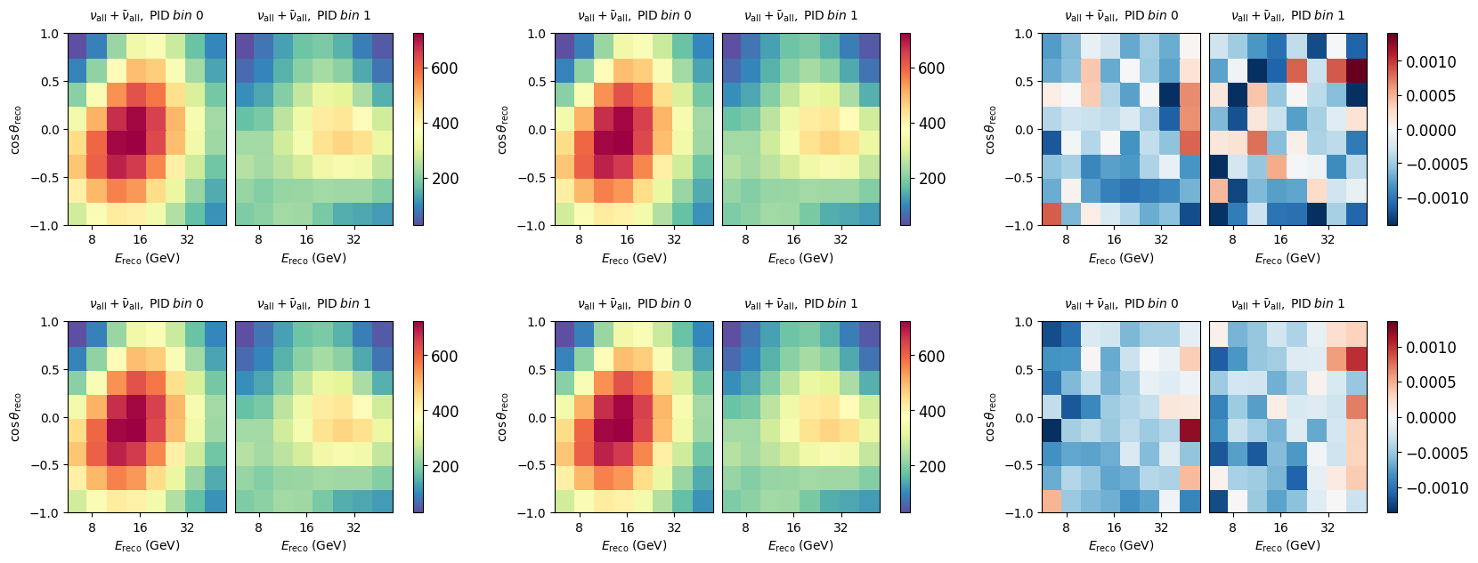
We can see that in this configuration we probably have fine enough grids, such that differences are at the sub-percent level. This may or may not be acceptable for the specific analysis you want to do.

fig, ax = plt.subplots(2, 3, figsize=(20, 7))
plt.subplots_adjust(hspace=0.5)

e = events.combine_wildcard('*')
m = mixed.combine_wildcard('*') 
g = grid.combine_wildcard('*') 

e.plot(ax=ax[0,0], title="Events")
m.plot(ax=ax[0,1], title="Mixed")
((e - m)/e).plot(ax=ax[0,2], symm=True)

e.plot(ax=ax[1,0], title="Events")
g.plot(ax=ax[1,1], title="Grid")
((e - g)/e).plot(ax=ax[1,2], symm=True)

(<Figure size 2000x700 with 18 Axes>,
 <Axes: title={'center': '${\\nu_{\\rm all}} + {\\bar\\nu_{\\rm all}},{\\;}{\\rm PID}{\\;}bin{\\;}0$'}, xlabel='$E_{\\rm reco} \\; \\left( \\mathrm{GeV} \\right)$', ylabel='$\\cos{\\theta}_{\\rm reco}$'>,
 <matplotlib.collections.QuadMesh at 0x7f760edadd10>,
 None)

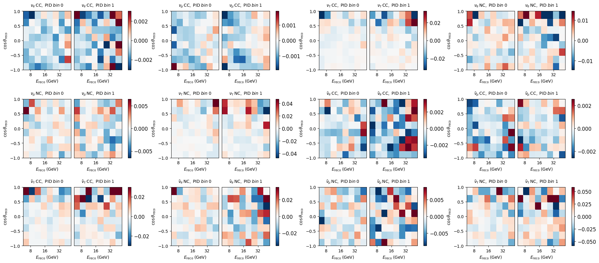
In depth comparison of single maps:

fig, axes = plt.subplots(3,4, figsize=(24,10))
plt.subplots_adjust(hspace=0.5)
axes = axes.flatten()

diff = (events - mixed) / (events + 1e-7)

for m, ax in zip(diff, axes):
    m.plot(ax=ax, symm=True)

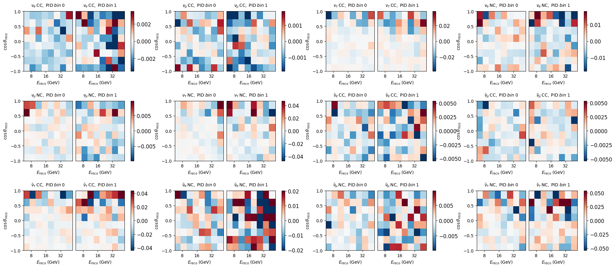
fig, axes = plt.subplots(3,4, figsize=(24,10))
plt.subplots_adjust(hspace=0.5)
axes = axes.flatten()

diff = (events - grid) / (events + 1e-7)

for m, ax in zip(diff, axes):
    m.plot(ax=ax, symm=True)